matlab相关函数使用
matlab 多目标最优 paretosearch
%main.m
clc
clear
fun=@(x)func_temp(x);
A=[-1 0;
   0 -1];
b=[-1 ;-2];
x=paretosearch(fun,2,A,b);
plot(x(:,1),x(:,2),'m*');
xlabel('x(1)');
ylabel('x(2)');
%func_temp.m
function f=func_temp(x)
    f(1)=x(1)+x(2);
    f(2)=2*x(2)+x(2);
end
三维空间中的汉字
text(x,y,z,'string')
绘制圆形
让原点在右上角,x轴向左,y轴向右
set(gca, 'XDir', 'reverse');  % x 轴方向反转
set(gca, 'YDir', 'reverse');  % y 轴方向反转
set(gca, 'XAxisLocation', 'top');  % x 轴在顶部
set(gca, 'YAxisLocation', 'right');  % y 轴在右侧
要沿 x 轴和 y 轴使用长度相等的数据单位
axis equal
求函数零点
- fzero
%fzero_test.m
function h=fzero_test(a)
    h=a^2-9;
end
%test.m
x0=[2 4];
fzero(@fzero_test,x0) % ans=3
matlab line 宽度,颜色,宽度
line([x1,x2],[y1,y2],'LineWidth', 2);
matlab利用最优化解决非线性微分方程
使用一次
x = optimvar('x');
y = optimvar('y');
x0=struct();
prob = optimproblem("Objective",peaks(x,y));

prob.Constraints.cons1 = x^2 + y^2 == 4;
prob.Constraints.cons2 = x^2 - y^2 == 0;
prob.Constraints.cons3 = x>=0;
prob.Constraints.cons4 = y>=0;
x0.x = 1;
x0.y = -1;
sol = solve(prob,x0)
约束不支持
当需要进行迭代时
x = optimvar('x');
y = optimvar('y');
x0=struct();
prob = optimproblem("Objective",peaks(x,y));

prob.Constraints.cons1 = x^2 + y^2 == 4;
prob.Constraints.cons2 = x^2 - y^2 == 0;
prob.Constraints.cons3 = x>=0;
prob.Constraints.cons4 = y>=0;
x0.x = 1;
x0.y = 0;
sol = solve(prob,x0)

%允许的
prob = optimproblem("Objective",peaks(x,y));
prob.Constraints.cons1 = x^2 + y^2 == 2;
prob.Constraints.cons2 = x^2 - y^2 == 0;
prob.Constraints.cons3 = x>=0;
prob.Constraints.cons4 = y>=0;
x0.x = 1;
x0.y = 0;
sol = solve(prob,x0)
参考
基于问题的有约束的非线性方程组 - MATLAB & Simulink - MathWorks 中国 求解优化问题或方程问题 - MATLAB solve - MathWorks 中国 求解优化问题或方程问题 - MATLAB solve - MathWorks 中国
求解非线性方程组
- fsolve()
matlab绘制datetime与因变量关系图
clc
clear
close all
fileName1_1="attach1_1.CSV";
data=readtable(fileName1_1)
% Assuming "data" is your array with missing values
data = rmmissing(data);%清理数据,删除数据丢失的行

time=datetime(table2array(data(:,1)),'InputFormat', 'yyyy-MM-dd HH:mm:ss');
T1=table2array(data(:,2));%table转数值数组
T2=table2array(data(:,3));

figure;
plot(time,T1);%打印
hold on;
plot(time,T2);%打印
hold on;
hold off;
matlab三维路径规划绘图.md
绘制立方体
hold on
grid on
plotcube([5 5 5],[ 2 2 2],.8,[1 0 0]);
plotcube([2 1 3],[ 10 10 10],.8,[144/256 144/256 144/256]);
axis([0 2000 0 2000 -200 600 ])   %设置图像的可视化范围

axis equal     % 图像坐标轴可视化间隔相等
xlabel('x');
ylabel('y');
plotcube([长,宽,高],[x,y,z坐标] , 透明度0~1 , [r , g ,b 0~1] );
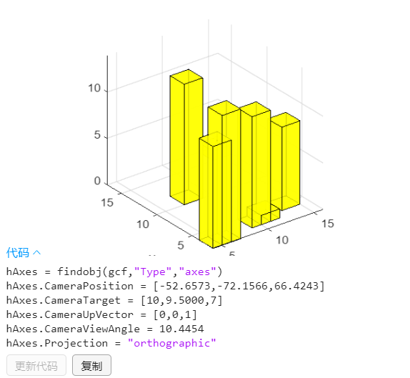
绘制立方柱
clc
clear
close all
hold on
grid on
rows=7;
place=randi(15,rows,2);
height=randi(15,rows,1);
for i=1:rows
    plotcube([2,2,height(i)],[place(i,:),0],0.8,[1 1 0]);
end

axis([0 2000 0 2000 -200 600 ])   %设置图像的可视化范围
axis equal     % 图像坐标轴可视化间隔相等
xlabel('x');ylabel('y');
自由视角
命令行输入 cameratoolbar
生成随机数矩阵
randi(max,rows,cols) 生成rows *cols的1~max的随机数矩阵
GPU加速
- gpuArray
a=[1 2 3;4 5 6 ; 7 8 9];%a在cpu里进行计算
b=gpuArray(a);%b在gpu里进行计算
- parfor 并行循环
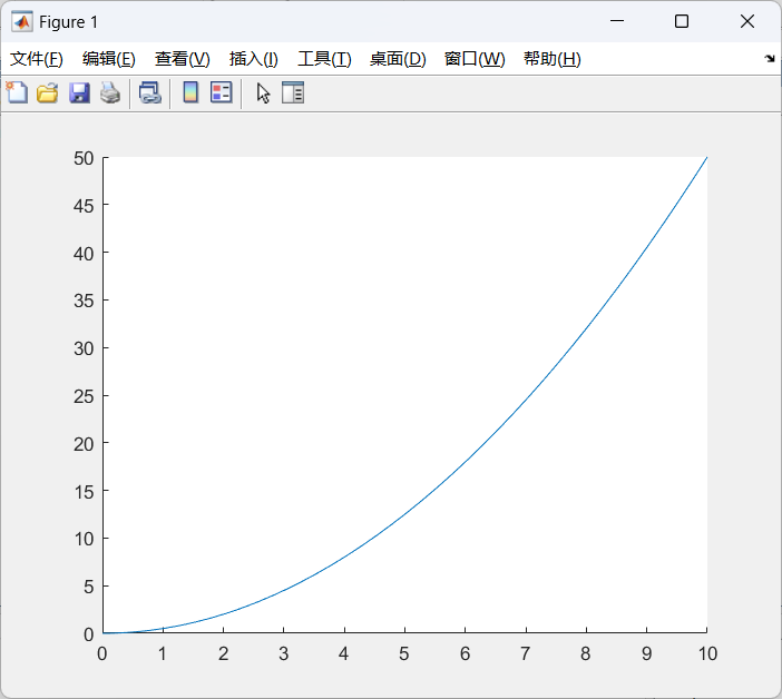
一阶微分方程
- 代码
%deal.m
function f=deal(t,y)
    f=(y^2-t-2)/(4*(t+1));
end
%test.m
[t,y]=ode45('deal',[0,2],0);
plot(t,y);
- 效果
- 带参数
%直线阻尼器的阻尼系数为常数
function f=myODE(t,x,a)    %a为直线阻尼系数
    k1=1025*9.8*pi*1^2;%静力回复系数
    k2=656.3616;%兴波阻力系数
    k3=80000;%弹簧刚度
    m1=2433;%振子质量
    m2=4866;%浮子质量
    m3=1335.535;%附加质量
    w=1.4005;%入射波浪频率
    f=6250;%垂荡激励力振幅 (N)
    %{
    x1 振子位移,向上为正
    x2 浮子位移,向上为正
    x3=diff(x1)
    x4=diff(x2)
    %}
    f=[
        x(3);
        x(4);
        ( -k3*(x(1)-x(2))-a*(x(3)-x(4)) )/(m1);
        ( f*cos(w*t)-k1*x(2)-k2*x(4)+k3*(x(1)-x(2))+a*(x(3)-x(4)) )/(m2+m3);
    ];
end
%main.m
[t,x]=ode45(@(t,x)myODE1(t,x,a),[0,40*2*pi/w],[0,0,0,0]);%括号一
可正常运行
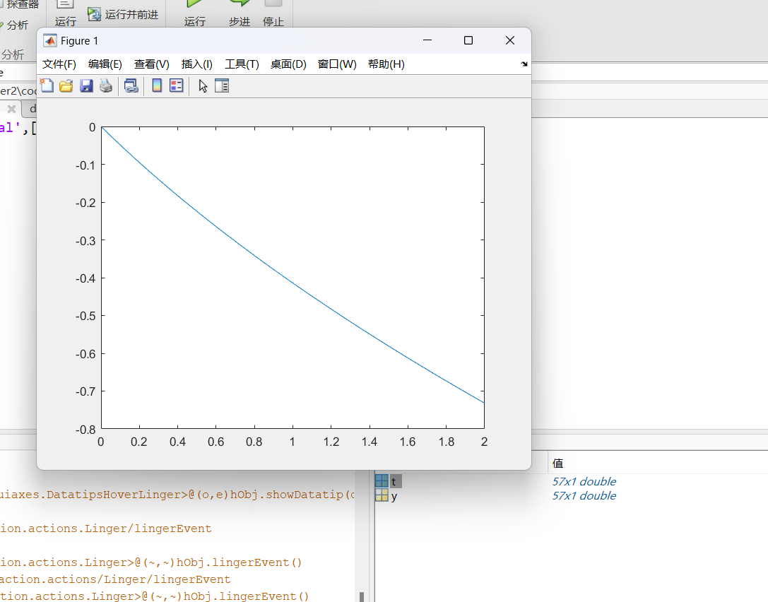
一阶微分方程组
function f=deal(t,y)
    f=[1;y(1)];
end
options = odeset('MaxStep', 1);
[t,y]=ode45('deal',[0,10],[0,0],options);
figure;
hold on;
plot(t,y(:,2));
- 效果
获取矩阵最大/最小元素及索引
[power_max,power_pos]=max(power_sum);
[maxVal, linearIndex] = max(power_sum(:));% 获取最小值和线性索引
[row, col] = ind2sub(size(power_sum), linearIndex);% 将线性索引转换为行列索引
绘制等高地形图,深度图,高度图
filename='attach.xlsx';
data=readtable(filename);

south_north=table2array(data(2:end,1));
west_east=table2array(data(1,2:end));
depth=table2array(data(2:end,2:end));

%海水深度
figure;
surf(repmat(south_north,1,201),repmat(west_east,251,1),depth);
font_size=15;
title("海水深度",FontSize=font_size+2);
xlabel("从南到北/NM",FontSize=font_size);
ylabel("从西到东/NM",FontSize=font_size);
zlabel("海水深度/m",FontSize=font_size);
shading interp;
saveas(gcf,'land_depth.png');

%海底形状
figure;
surf(repmat(south_north,1,201),repmat(west_east,251,1),-1*depth);
title("海底形状",FontSize=font_size+2);
xlabel("从南到北/NM",FontSize=font_size);
ylabel("从西到东/NM",FontSize=font_size);
zlabel("海拔高度/m",FontSize=font_size);
shading interp;
saveas(gcf,'land_shape.png');

%二维等高地平线
figure;

contourf(repmat(south_north,1,201),repmat(west_east,251,1),-1*depth);
title("海底等高地形图",FontSize=font_size+2);
xlabel("从南到北/NM",FontSize=font_size);
ylabel("从西到东/NM",FontSize=font_size);
zlabel("海水深度/m",FontSize=font_size);
colormap jet; % 设置颜色映射
colorbar; % 添加颜色图例
saveas(gcf,'land_same_height.png');
CSV导入数据,等高散点图
- 法一
filename='attach1.csv';
data=readtable(filename, 'VariableNamingRule', 'preserve');
x=table2array(data(:,2));
y=table2array(data(:,3));
z=table2array(data(:,4));

figure;
font_size=15;
scatter3(x, y, z, 20, z, 'filled'); % 36为点的大小,z用于指定颜色
xlabel("x/m",FontSize=font_size);
ylabel("y/m",FontSize=font_size);
zlabel("z/m",FontSize=font_size);
colorbar; % 添加颜色图例
saveas(gcf,"fast.png");
- 法二
filename='attach1.xls';
data=readtable(filename, 'VariableNamingRule', 'preserve');

wei=data.("任务gps 纬度");
jing=data.("任务gps经度");
无须再使用table2array
surf 光滑
clc;
clear;
filename='attach1.xlsx';
data=readtable(filename, 'VariableNamingRule', 'preserve');
data=table2array(data);
size=256;

surf(repmat(1:size,size,1)',repmat(1:size,size,1),data);
shading interp; % 启用插值着色